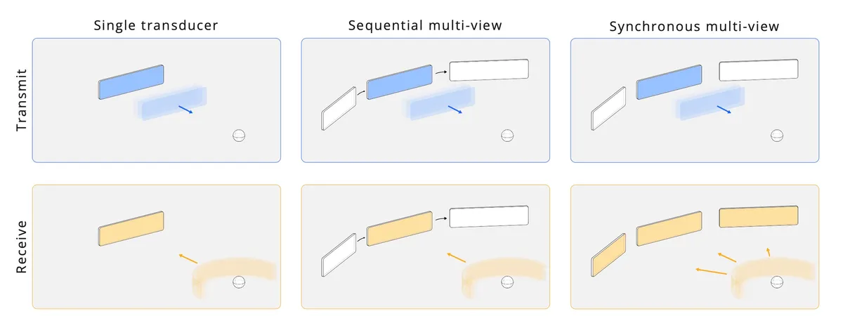
Typical diagnostic ultrasound imaging uses a single transducer to both transmit a pulse and receive back-scattered signal. Multi-view ultrasound involves the collection and aggregation of more information into a single image. Data collection can be sequential, involving a series of single transducer images, or it can be synchronous, where multiple transducers transmit and/or receive simultaneously.
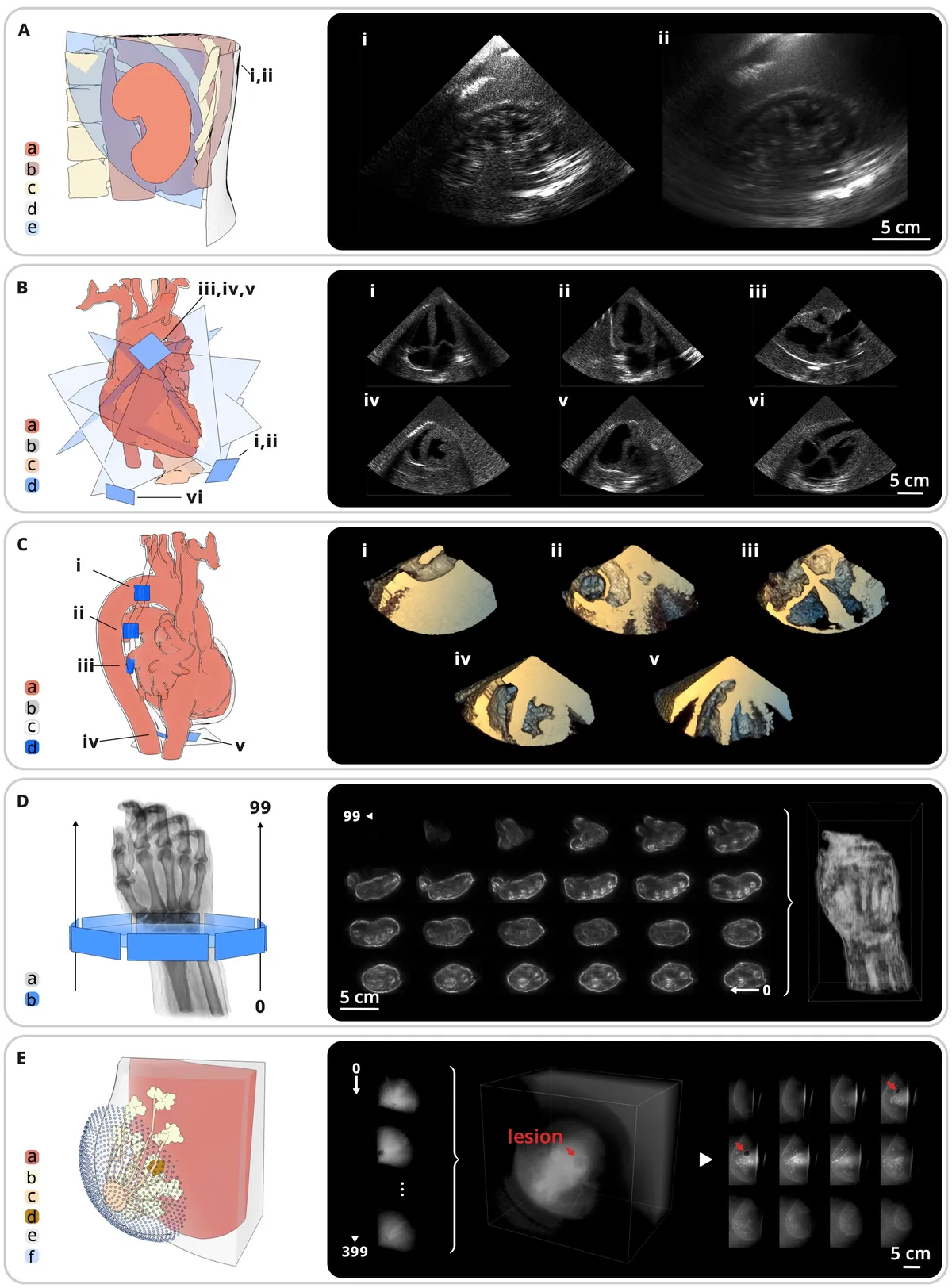
Five in vivo experiments simulated in MUSiK. (A) Simulated longitudinal kidney scan using (i) a focused transducer and (ii) a plane wave transducer. (a. kidney cortex, b. muscle, c. bone, d. body surface, e. transducer sweep) (B) Simulated 2D transesophageal echocardiography exam from 6 standard views of the heart, obtained on 3 windows. (a. blood pool, b. myocardium and vasculature, c. esophagus, d. transducer and sweep) (C) Simulated 3D transesophageal echocardiography exam from 5 3D views of the heart. (a. blood pool, b. myocardium and vasculature, c. esophagus, d. transducer) (D) Simulated 2.5D ultrasound tomography experiment imaging the forearm. (a. tissue density, b. transducer) (E) Simulated 3D ultrasound tomography experiment imaging the breast. (a. muscle, b. mammary lobe, c. mammary duct, d. anechoic tumor, e. body surface, f. transducer)
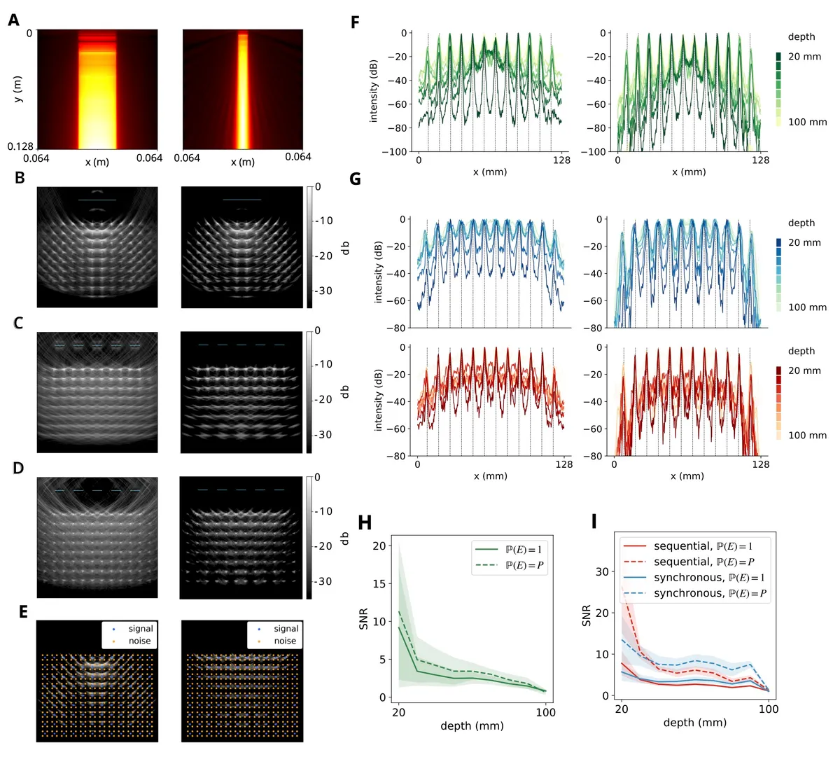
Coherent compounding reconstruction benefits from excitation compensation broadly. (A) Maximum pressure amplitude computed analytically for a single θ = 0 pulse from the 40 mm transducer and the 10 mm transducer. This was used for excitation compensation in the following single- and multi-view experiments. (B–D) Single transducer (B), multi-view setup with sequential compounding (C), and multi-view setup with synchronous compounding (D) images, without (left) and with (right) excitation compensation applied during reconstruction. (E) Points denoting scatterers and background, used to measure SNR. (F, G) Lateral PSFs as a function of imaging depth for single-view (F), sequential multi-view (G, upper), and synchronous multi-view (G, lower) imaging, without (left) and with (right) excitation compensation. (H) SNR as a function of depth for a single transducer. Shaded regions denote one standard deviation from the mean. (I) SNR as a function of depth for a multi-view setup.
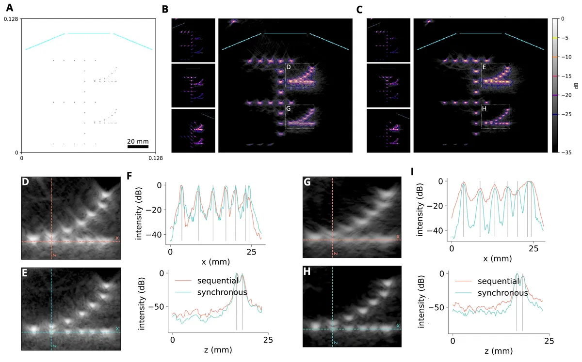
A multi-view ultrasound experiment to measure resolution in vitro simulated in MUSiK. (A) The simulated 3-transducer aperture and phantom. (B) Images obtained with a sequential acquisition where each transducer transmits and receives independently (left) and their combined reconstruction (right). (C) Images obtained using a synchronous acquisition where each transducer transmits independently, but all transducers are included in the receive aperture (left), and their combined reconstruction (right). (D, E, F) Inset images for the near field resolution phantom for (D) sequential and (E) synchronous acquisitions, with (F) the lateral and longitudinal point-spread-functions plotted. (G, H, I) Inset images for the far field resolution phantom for (G) sequential and (H) synchronous acquisitions and (I) their lateral and longitudinal point-spread-functions.